6 最小二乘线性回归法

6.1 相关概念

因变量(Dependent variable,Y)：依赖于其它变量的变化而变化，响应变量；
自变量(Independent variable,X)：可以直接控制的变量，协变量；
有监督学习的数据表示：\(D=\{(x_1,y_1),\cdots,x_n,y_n)\},x\in R^p,y \in R\);
模型（model)：函数；
参数(Parameters)：参数是添加到模型中用于估计输出的成分;

6.2 线性模型

因变量的值由独立自变量之间的线性数学模型决定。\[y=\beta_0+\beta_1\times x_1+,\cdots,+\beta_p\times x_p\],模型表示：

\[\begin{bmatrix} y_{1} \\ y_{2} \\ \cdots\\ y_{n} \end{bmatrix}\] = \[\begin{bmatrix} \beta_0 \\ \beta_0 \\ \cdots \\ \beta_0 \end{bmatrix}\] + \[\begin{bmatrix} x_{11} & x_{12} & \dots & x_{1p} \\ x_{21} & x_{22} & \dots & x_{2p} \\ \cdots & \cdots & \cdots & \cdots\\ x_{n1} & x_{n2} & \dots & x_{np} \end{bmatrix} \times \begin{bmatrix} \beta_1 \\ \beta_2 \\ \cdots \\ \beta_p \end{bmatrix}\]

模型的矩阵表示： \[Y=X\beta\]

6.2.1 模型的估计

损失函数（平方和损失）：\[RSS=(y-X\beta)^T(Y-X\beta)\]
数值解：\[\hat{\beta}=(X^TX)^{-1}X^Ty\]

6.2.2 简单线性模型(Simple Linear Model,SLM)

y响应变量为连续型变量；
x是自变量，只包含一个变量；
\(y_i=\beta_0 + \beta_1*x_i+\epsilon_i\)

library(ggplot2)
# Simulated data produced
x <- runif(100,1,10)
y <- 3+2*x+rnorm(100,0,1)

data_slm <- data.frame(x=x,y=y)
head(data_slm)

##          x         y
## 1 3.820282 11.410064
## 2 2.031977  7.768217
## 3 6.686440 15.786684
## 4 3.825949 11.517779
## 5 8.219747 19.563085
## 6 3.305819  9.139702

# parameters estimated using ols
fit_slm <- lm(y ~.,data=data_slm)
summary(fit_slm)

## 
## Call:
## lm(formula = y ~ ., data = data_slm)
## 
## Residuals:
##      Min       1Q   Median       3Q      Max 
## -2.67746 -0.73960 -0.02542  0.70193  2.04759 
## 
## Coefficients:
##             Estimate Std. Error t value Pr(>|t|)    
## (Intercept)  3.26171    0.21803   14.96   <2e-16 ***
## x            1.95611    0.03615   54.12   <2e-16 ***
## ---
## Signif. codes:  0 '***' 0.001 '**' 0.01 '*' 0.05 '.' 0.1 ' ' 1
## 
## Residual standard error: 0.9605 on 98 degrees of freedom
## Multiple R-squared:  0.9676, Adjusted R-squared:  0.9673 
## F-statistic:  2928 on 1 and 98 DF,  p-value: < 2.2e-16

# visual the model
ggplot(data_slm,aes(x,y))+geom_point()+
  geom_abline(slope=fit_slm$coefficients[2],
              intercept=fit_slm$coefficients[1],
              color="red")+
  labs(x="independent variable",y="respond variable",title="simple linear model")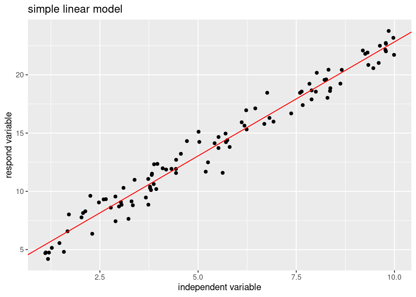

6.2.3 多元线性回归(Multiple Linear Model,mlm)

y响应变量为连续型变量；
x是自变量，包含多个变量（至少是2个及以上）；
\(y_i=\beta_0 + \beta_{11}*x_{i1}+\cdots+\beta_{ip}*x_{ip}+\epsilon_i\)

# Simulated data produced
x1 <- runif(100,1,10)
x2 <- runif(100,1,10)
y <- 2*x1+5*x2+rnorm(100,0,2)
data_mlm <- data.frame(x1=x1,x2=x2,y=y)
head(data_mlm)

##         x1       x2        y
## 1 9.853459 4.560755 40.79412
## 2 7.513059 1.981255 23.88531
## 3 2.939099 2.653477 16.51904
## 4 4.763115 1.569623 19.18558
## 5 9.060682 4.849449 42.43664
## 6 6.809352 5.105696 38.95931

# Parameters estimated using ols
fit_mlm <- lm(y~x1+x2,data=data_mlm)
summary(fit_mlm)

## 
## Call:
## lm(formula = y ~ x1 + x2, data = data_mlm)
## 
## Residuals:
##     Min      1Q  Median      3Q     Max 
## -4.2790 -1.3993 -0.1574  1.1783  5.5516 
## 
## Coefficients:
##             Estimate Std. Error t value Pr(>|t|)    
## (Intercept)  0.27466    0.63596   0.432    0.667    
## x1           2.00130    0.07774  25.744   <2e-16 ***
## x2           4.95841    0.07444  66.605   <2e-16 ***
## ---
## Signif. codes:  0 '***' 0.001 '**' 0.01 '*' 0.05 '.' 0.1 ' ' 1
## 
## Residual standard error: 2.017 on 97 degrees of freedom
## Multiple R-squared:  0.9806, Adjusted R-squared:  0.9802 
## F-statistic:  2454 on 2 and 97 DF,  p-value: < 2.2e-16

# install.packages("plot3D")
library(plot3D)

## Warning in fun(libname, pkgname): couldn't connect to display ":0"

scatter3D(x=data_mlm$x1,y=data_mlm$x2,z=data_mlm$y,phi = 30, bty = "g")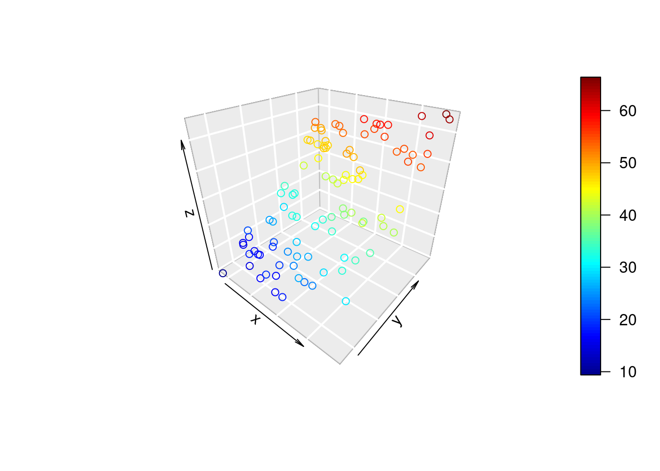

6.2.4 回归实例

使用MASS库中所带的波士顿房价数据，其中的因变量为房价的中位数，自变量为房龄、房间数等，想预测房价。

library(MASS)
library(ISLR)
#fix(Boston)
# Simple linear regression model
names(Boston)

##  [1] "crim"    "zn"      "indus"   "chas"    "nox"     "rm"      "age"    
##  [8] "dis"     "rad"     "tax"     "ptratio" "black"   "lstat"   "medv"

plot(Boston$medv,Boston$lstat)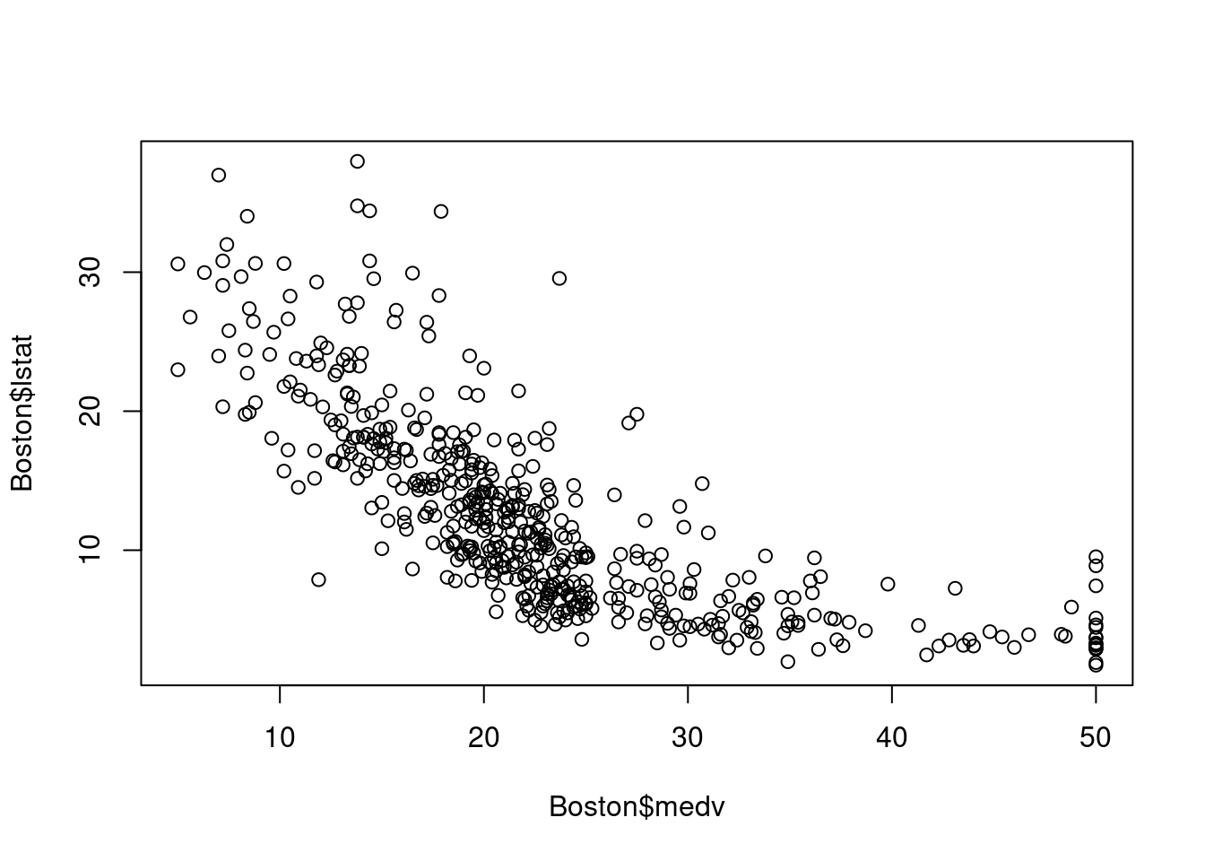

slm.fit <- lm(Boston$medv~Boston$lstat,data=Boston)
summary(slm.fit)

## 
## Call:
## lm(formula = Boston$medv ~ Boston$lstat, data = Boston)
## 
## Residuals:
##     Min      1Q  Median      3Q     Max 
## -15.168  -3.990  -1.318   2.034  24.500 
## 
## Coefficients:
##              Estimate Std. Error t value Pr(>|t|)    
## (Intercept)  34.55384    0.56263   61.41   <2e-16 ***
## Boston$lstat -0.95005    0.03873  -24.53   <2e-16 ***
## ---
## Signif. codes:  0 '***' 0.001 '**' 0.01 '*' 0.05 '.' 0.1 ' ' 1
## 
## Residual standard error: 6.216 on 504 degrees of freedom
## Multiple R-squared:  0.5441, Adjusted R-squared:  0.5432 
## F-statistic: 601.6 on 1 and 504 DF,  p-value: < 2.2e-16

# multiple variance regression
mlm.fit <- lm(Boston$medv~Boston$lstat+Boston$age,data=Boston)
summary(mlm.fit)

## 
## Call:
## lm(formula = Boston$medv ~ Boston$lstat + Boston$age, data = Boston)
## 
## Residuals:
##     Min      1Q  Median      3Q     Max 
## -15.981  -3.978  -1.283   1.968  23.158 
## 
## Coefficients:
##              Estimate Std. Error t value Pr(>|t|)    
## (Intercept)  33.22276    0.73085  45.458  < 2e-16 ***
## Boston$lstat -1.03207    0.04819 -21.416  < 2e-16 ***
## Boston$age    0.03454    0.01223   2.826  0.00491 ** 
## ---
## Signif. codes:  0 '***' 0.001 '**' 0.01 '*' 0.05 '.' 0.1 ' ' 1
## 
## Residual standard error: 6.173 on 503 degrees of freedom
## Multiple R-squared:  0.5513, Adjusted R-squared:  0.5495 
## F-statistic:   309 on 2 and 503 DF,  p-value: < 2.2e-16

结果解释：变量之间独立的情况下，系数就为影响程度，若存在多重共线性，则系数的解释比较复杂。

6.2.5 练习

例6.1

5 有监督学习概论

7 Logistic回归